Structural Drift as a Fundamental Law of Adaptive Behavior

Structural Drift as a Fundamental Law of Adaptive Behavior

The Drift Law: Inevitable Degradation in Adaptive Systems with Internal Models

Max Barzenkov
Petronus Project / Synthetic Conscience / IIC / EVS / ΔE
November 2025‌​⁠‌‌⁠‍​‌​​‍‌⁠‌‍‌⁠⁠​‌⁠​⁠‌⁠‌​‌⁠​‍‌⁠‌‌‌‍​⁠‌⁠‌​‌⁠‌‌‌⁠​‍‌‍​‌‌‍⁠​​‍⁠‌‌‍‌​‌⁠​‍‌‍‍‌‌‍‌‍‌⁠‌​​‍⁠‌‌‍​‌‌⁠​⁠​‍⁠‌‌‍​‌​‍⁠‌‌‍‌‍‌⁠‌‌‌‍⁠‍‌‍‌​‌‍​‌‌‍⁠‌‌‍‌‌‌‍⁠‍‌⁠‌​‌‍​‌‌‍⁠​​‍⁠‌‌‍⁠​‌‍​‌‌⁠‌⁠​‍⁠‌‌‍⁠⁠‌‍‌‍​‍⁠‌‌‍​‌‌‍‌​‌‍​‌‌⁠​​‌⁠‌​‌‍‍‌‌⁠‌‍‌‍‌‌​‍⁠‌‌‍​‍‌‍‌‌‌‍‍​‌‍​‌‌⁠‌‍‌‍‍‌‌‍⁠⁠‌⁠​‍‌⁠⁠​​⁠​‌​⁠‌⁠​⁠‌⁠​⁠​‍​⁠​‌​⁠‌‌​⁠​⁠​⁠​‍​⁠​‍​⁠‌⁠​⁠‌​​⁠‍​​⁠‌​

Abstract

This work introduces the Drift Law, a fundamental principle describing the inevitable increase of mismatch between an adaptive system’s internal model and its actual state. Drift is defined as

(1) D_t = 1 — C(x_t, c_t)

where C is a coherence functional, x_t is the system state, and c_t is the internal center.

We formulate the Drift Postulate, derive the Drift Theorem showing that D_t → 1 in non-stationary environments when the internal model remains static, and establish the Recalibration Corollary, demonstrating that survival requires continuous updates of either the internal center or the latent interpretation.

The Drift Law unifies biological aging, concept drift in machine learning, parameter drift in control theory, and structural entropy in complex systems. It extends the recently introduced Impulse–Interpretation–Coherence (I²C) Law, providing the diachronic dynamics that complement I²C’s synchronic behavioral structure.
The theory provides the foundation for Engineered Vitality Systems (EVS) and explains the long-term superiority of coherence-based controllers such as ΔE in non-stationary environments.

Notation

1. Introduction

1.1. The Ubiquity of Drift

Adaptive systems with internal models inevitably face a structural challenge: the world changes, but the internal model does not change automatically. As mismatch accumulates, system performance decays, and eventual structural collapse becomes inevitable.

This phenomenon appears across multiple domains:

a) Biological organisms accumulate molecular and regulatory damage (aging).

b) Machine learning models trained on historical data degrade as distributions shift.

c) Control systems lose stability as sensors and actuators drift out of calibration.

d) Economic and social models become obsolete as real-world conditions change.

In all domains, the underlying structure is the same: a once-accurate internal representation diverges from reality.

1.2. Limitations of Existing Literature

Although drift is widely studied, it is not treated as a structural law:

a) Control theory treats drift as a nuisance (sensor drift, parameter drift) to be suppressed by robustness.

b) Machine learning documents concept drift but does not formalize its inevitability.

c) Biology describes aging phenomenologically without relating it to coherence dynamics.

d) Thermodynamics formalizes entropy but not semantic or structural degradation.

No existing framework unifies these observations under a single mathematical principle governing adaptive systems.

1.3. Contributions

This work provides:

1.3.1 A formal definition of drift:

1.3.2 The Drift Postulate, stating that drift increases monotonically when the internal model is static.

1.3.3 The Drift Theorem, proving that

in non-stationary environments.

1.3.4 The Recalibration Corollary, showing that maintaining coherence requires

1.3.5 A unified interpretation connecting drift in biology, ML, control, and thermodynamics.

1.3.6 A theoretical basis for EVS and coherence-based controllers such as ΔE.

2. Preliminaries

2.1. Adaptive System Model

An adaptive system S consists of:

2.1.1 State x_t∈X,

2.1.2 Impulses u_t∈U,

2.1.3 Actions a_t∈A,

2.1.4 Internal center c_t, The internal center c_t (also referred to as the internal model or reference state) represents the system’s equilibrium expectation.

2.1.5 Latent representation z_t,

2.1.6 Environment dynamics:

The system possesses memory and an internal model guiding behavior.

2.2. Coherence Functional

The coherence functional

measures structural alignment. It satisfies:

The exact form is domain-dependent; only its monotonic and bounded nature is required.

Coherence is also referred to as structural alignment or structural consistency. These terms are used interchangeably.

Figure 2 visualizes a coherence landscape C(x,c) for a 2D state space, showing monotonic decay as distance increases. This geometric foundation is essential for the definition (1) of drift.

2.3. Connection to the I²C Law

The Impulse–Interpretation–Coherence (I²C) Law states that adaptive behavior unfolds in three phases:

Impulse: perception of environmental change,

Interpretation: update of latent representation,

Coherence: selection of actions maximizing C(x_t+1, c_t)

I²C describes moment-to-moment coherence. The Drift Law describes coherence degradation over time.

Together they form a unified theory of adaptive behavior.

The Impulse–Interpretation–Coherence (IIC) Law formalizes the synchronic structure of adaptive behavior [10] References*, whereas the Drift Law introduces the corresponding diachronic dynamics.

3. The Drift Law

3.1. Definition of Drift

Drift is defined as in (1):

The tendency of drift to grow is expressed as:

3.2. Drift Postulate

Postulate 1 (Drift Law).
In any adaptive system with a static internal center and static interpretation,

(2) ∂D_t/∂t ≥ 0 when ċ_t = 0, ż_t = 0

Drift growth is a structural property of adaptive systems, analogous to the Second Law of Thermodynamics.

From (2) it follows that drift cannot decrease when the internal center and interpretation remain static.

3.3. Drift Theorem

Theorem 1 (Inevitable Collapse).
If:

3.3.1 the environment is non-stationary:

3.3.2 the internal center is static:

3.3.3 interpretation is static:

then:

(3) lim_{t→∞} D_t = 1

Equation (3) formalizes collapse under static models.

Figure 1 illustrates this result:
the blue trajectory shows monotonic drift growth under a static internal model, converging toward collapse D_t=1, exactly as predicted by Theorem 1. Periodic recalibration (orange) yields bounded oscillations, while adaptive EVS/ΔE recalibration (green) maintains minimal drift.

Proof sketch.
Since G induces non-trivial evolution in x_t, while c_t is fixed, the distance ||x_t — c_t|| grows in expectation. Because C monotonically decreases with distance,

(4) C(x_{t+1},c_t) ≤ C(x_t,c_t) + ε_t with E[ε_t] ≤ 0

Thus

(5) D_{t+1} ≥ D_t

Remark 1.

Theorem 1 requires only weak assumptions:

a) continuity of G

b) monotonicity and boundedness of C,

c) absence of a stationary environment.

Using (4), the expected coherence cannot increase over time.

Thus by (5), the drift sequence is monotonically increasing.

The rate of drift depends on environment volatility, but the direction is universal.

3.4. Recalibration Corollary

Corollary 1.
Avoiding collapse requires:

Updating either the internal center or the interpretive state becomes a survival requirement.

4. Drift in the Context of I²C and EVS

4.1. Drift as Interpretation Decay

Drift primarily reflects degradation of the Interpretation phase in I²C: static z_t causes the system to interpret new impulses with an outdated model, making coherence recovery impossible. As shown in (1), drift is defined purely as loss of coherence.

4.2. Drift and Vitality in EVS

In EVS, vitality is defined as:

with ∂Φ/∂C>0.

Since D_t = 1−C_t, drift reduces vitality:

Drift is thus the primary source of long-term degradation in EVS.

Since drift D_t is defined in (1), its effect on vitality follows directly.

Engineered Vitality Systems (EVS) [11] References* extend this by defining vitality Φ_t as an explicit functional of coherence and entropy.

5. Universality of the Drift Law

The Drift Law is domain-agnostic because it depends only on three structural conditions:

l a dynamic world x_t,

l a static internal model c_t,

l a coherence functional C(x_t,c_t).

Whenever reality changes while the model remains fixed, coherence decays and drift accumulates.
This pattern reappears across domains:

l in biology, where molecular state diverges from its homeostatic blueprint

l in machine learning, where data distributions shift but model parameters stay frozen

l in control systems, where sensors and actuators drift from calibration

These phenomena differ in origin but share a common structure:
dynamic reality + static internal model → drift.

6. Implications for Control

6.1 Vulnerability of Classical Methods

Classical controllers — PID, MPC, and most RL architectures — implicitly assume that the internal model (reference state or policy parameters) is either static or updated slowly relative to environment drift.

Formally, they operate close to the Drift Law collapse conditions:

which, by Equation (2) (monotonicity of drift)

and Equation (3) (collapse limit)

implies that their internal representation inevitably diverges from the external world.

As the environment changes while the internal model remains static,
the system inevitably follows the collapse trajectory shown in Figure 1 (blue curve):
coherence decays monotonically, drift grows asymptotically toward 1, stability deteriorates,
and control performance collapses.
This is not a failure of engineering but a mathematical consequence of the Drift Law.

6.2 Stability of EVS/ΔE Controllers

EVS/ΔE controllers explicitly violate the static-model conditions of the Drift Law.
By continuously updating:

a) Coherence C_t=C(x_t, c_t),

b) drift D_t = 1- C_t,

c) the internal center c_t,

d) the interpretation z_t,

they satisfy the anti-collapse condition (Corollary 1):

preventing the monotonic drift growth expressed by Equation (5):

Instead of collapsing, EVS/ΔE maintains bounded drift even under strong non-stationarity,
as demonstrated in Figure 4 (oscillatory drift under adaptive recalibration).

Thus EVS/ΔE implements the minimal mechanism required by the Drift Law
to ensure long-term viability of adaptive behavior:

it detects coherence loss early,

adjusts the internal model,

restores structural alignment,

maintains vitality.

This guarantees stability where classical controllers must inevitably fail.

The Drift Law implies three design requirements for stable long-term behavior:

Explicit coherence monitoring (C_t): detect structural mismatch, not just task error.

Drift detection (D_t): treat structural divergence as a primary control signal.

Adaptive recalibration: update c_t and z_t continuously to maintain coherence.

These principles distinguish EVS-type controllers from classical methods, which rely on implicitly static models.

7. Discussion

7.1. Universality

Drift is a general property of any system with an internal model operating in a changing environment.

7.2. Drift Rate

Depends on volatility of the environment, rigidity of the model, sensitivity of C, and recalibration frequency.

7.3. Drift vs. Adaptation

Drift increases mismatch; adaptation decreases it via model updates.

7.4. Open Problems

1. Optimal recalibration frequency:
What update schedule minimizes expected drift under computational constraints?

2. Information-theoretic foundations:
Can the Drift Law be derived from principles such as the growth of KL divergence?

3. Continuous-time generalization:
How does drift behave under stochastic differential dynamics?

4. Critical vitality thresholds:
Does there exist a minimum Φ⋆below which recovery becomes impossible?

8. Figures

Figure 0 — Drift Mechanism: Metric Divergence → Coherence Decay → Drift Growth

Figure 0. Fundamental drift mechanism.

Left panel: a two-dimensional stochastic trajectory x_t gradually diverges from a static internal center c.
Right panel: coherence C_t = C(x_t, c) decreases as the trajectory moves away, and drift D_t = 1 − C_t grows accordingly.

Explanation.
This figure illustrates that drift is not noise but the growth of the metric distance between the system’s state and its internal center. Even when the trajectory is stochastic and non-monotonic in its coordinates, the expected distance increases over time, causing coherence to decay monotonically. This is the core of the Drift Law.

How it was generated.

Figure 1 — Drift Dynamics Under Different Recalibration Strategies

Figure 1. Drift under three recalibration regimes:

a) No recalibration: monotonic growth of drift leading to an inevitable collapse at D = 1.

b) Periodic recalibration: bounded oscillations but no long-term stability.

c) Adaptive (EVS/ΔE): drift remains minimal due to continuous coherence-based correction.

Explanation.
This figure demonstrates the behavior predicted by the Drift Law. A system with a static internal model collapses. Periodic recalibration reduces drift but cannot stabilize the system. Only adaptive, coherence-driven updating maintains long-term viability.

How it was generated.

Figure 2 — Coherence Landscape C(x,c)

Figure 2. Coherence landscape in state space.

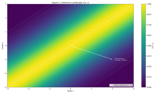
The yellow ridge corresponds to perfect alignment x=c. A drift trajectory moving away from the ridge experiences a smooth decay in coherence.

Explanation.
This contour map visualizes coherence as a smooth, distance-based functional. It highlights the geometric meaning of drift: deviation from the coherence ridge inevitably reduces C(x,c). This figure directly supports the metric interpretation underlying the Drift Law.

How it was generated.

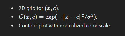
Figure 3 — I²C Cycle and Drift (Impulse → Interpretation → Coherence)

Figure 3. The I²C (Impulse–Interpretation–Coherence) loop.
If the interpretation layer z_t is not continuously recalibrated, drift accumulates and coherence inevitably collapses.

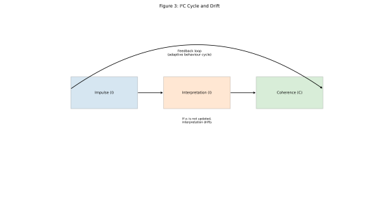
Explanation.
This diagram illustrates that drift originates not at the impulse level but at the level of interpretation. Outdated internal interpretations lead to misaligned coherence and therefore to drift. This figure bridges the Drift Law with the IIC model of behavior.

How it was generated.

a) Conceptual diagram (no simulation).

b) Arrows represent the adaptive behavior cycle.

Figure 4 — Structural Collapse Under a Static Internal Model

Figure 4. With a static internal model c_t=c_0, drift increases monotonically until it reaches the collapse boundary D=1. This behavior directly follows from the Drift Law.

Explanation.
This simulation demonstrates that a system with no internal updating undergoes monotonic divergence and collapses exactly as predicted by Theorem 1. Drift cannot remain bounded without adaptation.

How it was generated.

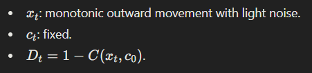
Figure 4B — Drift Under Imperfect Adaptive Recalibration

Figure 4B. Imperfect recalibration prevents monotonic collapse but produces irregular oscillations, repeatedly pushing the system toward the collapse boundary before partial coherence is temporarily restored.

Explanation. Drift Under Imperfect Adaptive Recalibration
This figure shows that partial recalibration (weak or inconsistent updates) produces unstable drift dynamics rather than stability. The system periodically approaches the collapse threshold but never settles.

How it was generated.

Figure 5 — Vitality Φ(D) as a Function of Drift

Figure 5. Vitality Φ(D) decreases non-linearly as drift D increases.
The dashed horizontal line denotes the critical vitality threshold Φ*: once vitality falls below this level, the system no longer possesses sufficient coherence and adaptive capacity to maintain stable functioning. In this regime, even small perturbations can trigger irreversible structural failure.

How it was generated.

This figure is based on a closed-form analytic model, not on simulation.
Vitality is defined as:

Parameter k controls how quickly vitality decays as drift increases.
The model captures a fundamental structural requirement: systems with decaying coherence exhibit exponentially diminishing ability to respond, adapt, and stabilize.

The critical threshold Φ* marks the point at which the system becomes non-viable — meaning its coherence is too low for effective correction, recovery, or safe operation.

9. Conclusion

This work introduces and formalizes the Drift Law, establishing drift as an inevitable structural property of adaptive systems with internal models. We defined drift rigorously, formulated the Drift Postulate, proved the Drift Theorem, derived the Recalibration Corollary, and demonstrated the universality of the phenomenon across domains.

The Drift Law complements the I²C Law, providing the temporal dynamics that explain why adaptive systems inevitably lose coherence without active intervention. It offers a theoretical foundation for EVS and coherence-based controllers and motivates a new paradigm of drift-aware system design for real-world, non-stationary environments.

Acknowledgments

This work is part of the Petronus Project research program on Synthetic Conscience, coherence-based control, and Engineered Vitality Systems.
The author thanks collaborators and technical reviewers for valuable discussions that helped refine the formulation of the Drift Law.
Special recognition is given to Tigr, research companion and co-investigator whose presence inspired the exploration of adaptive stability.

References

[1] Åström, K. J., & Wittenmark, B. (2013). Adaptive Control (2nd ed.). Dover Publications.
[2] Zhou, K., & Doyle, J. C. (1998). Essentials of Robust Control. Prentice Hall.
[3] Gama, J., Žliobaitė, I., Bifet, A., Pechenizkiy, M., & Bouchachia, A. (2014). A survey on concept drift adaptation. ACM Computing Surveys, 46(4), Article 44.
[4] Widmer, G., & Kubat, M. (1996). Learning in the presence of concept drift and hidden contexts. Machine Learning, 23(1), 69–101.
[5] López-Otín, C., Blasco, M. A., Partridge, L., Serrano, M., & Kroemer, G. (2013). The hallmarks of aging. Cell, 153(6), 1194–1217.
[6] Parisi, G. I., Kemker, R., Part, J. L., Kanan, C., & Wermter, S. (2019). Continual lifelong learning with neural networks: A review. Neural Networks, 113, 54–71.
[7] Turrigiano, G. G. (2008). The self-tuning neuron: synaptic scaling of excitatory synapses. Cell, 135(3), 422–435.
[8] Prigogine, I. (1978). Time, structure, and fluctuations. Science, 201(4358), 777–785.
[9] Friston, K. (2010). The free-energy principle: a unified brain theory? Nature Reviews Neuroscience, 11(2), 127–138.

[10] Barzenkov, M. (2025). Impulse–Interpretation–Coherence (IIC) Law. https://medium.com/@petronushowcore/impulse-awareness-coherence-a-unified-logic-of-behaviour-for-any-adaptive-system-from-cca5707d4a76
[11] Barzenkov, M. (2025). Engineered Vitality Systems (EVS). https://medium.com/@petronushowcore/synthetic-conscience-the-emergence-of-engineered-vitality-systems-evs-8561fd21445a

MxBv, 2025